The SafetySkills system is now using a time format for “Total Time” that allows for time greater than 24 hours to be tracked for one assignment/completion. This was needed for courses such as Authorized OSHA 30 and other offline training to be able to reflect full training time. In order to accommodate this request, the “Total Time” field had to be reformatted and is no longer a traditional time value at the database level.
This has created some additional steps to calculate time in Excel, or other programs. The LMS will populate the total minutes in the system for you. The total minutes can be divided by 60 to give you hours quickly. If you have the need to make other calculations, please follow these steps to reformat the time in Excel.
Start by exporting the report data from the system. The format you choose will determine the steps needed to update the time values to be able to run calculations. The CSV file (.csv) will automatically transform any time over 100 hours to a time format. This means that you will only need to follow these instructions for times of 0099:59:59 or less. If you export the Excel option (.xlsx) you will need to perform actions on all the time values before you can calculate on the times.
Open the file in Excel
Sort the “Total Time” from “Z to A.” This will bring the larger times to the top.
On the right side of the “Total Time,” add 2 new columns. Right click on the column header, select Insert.
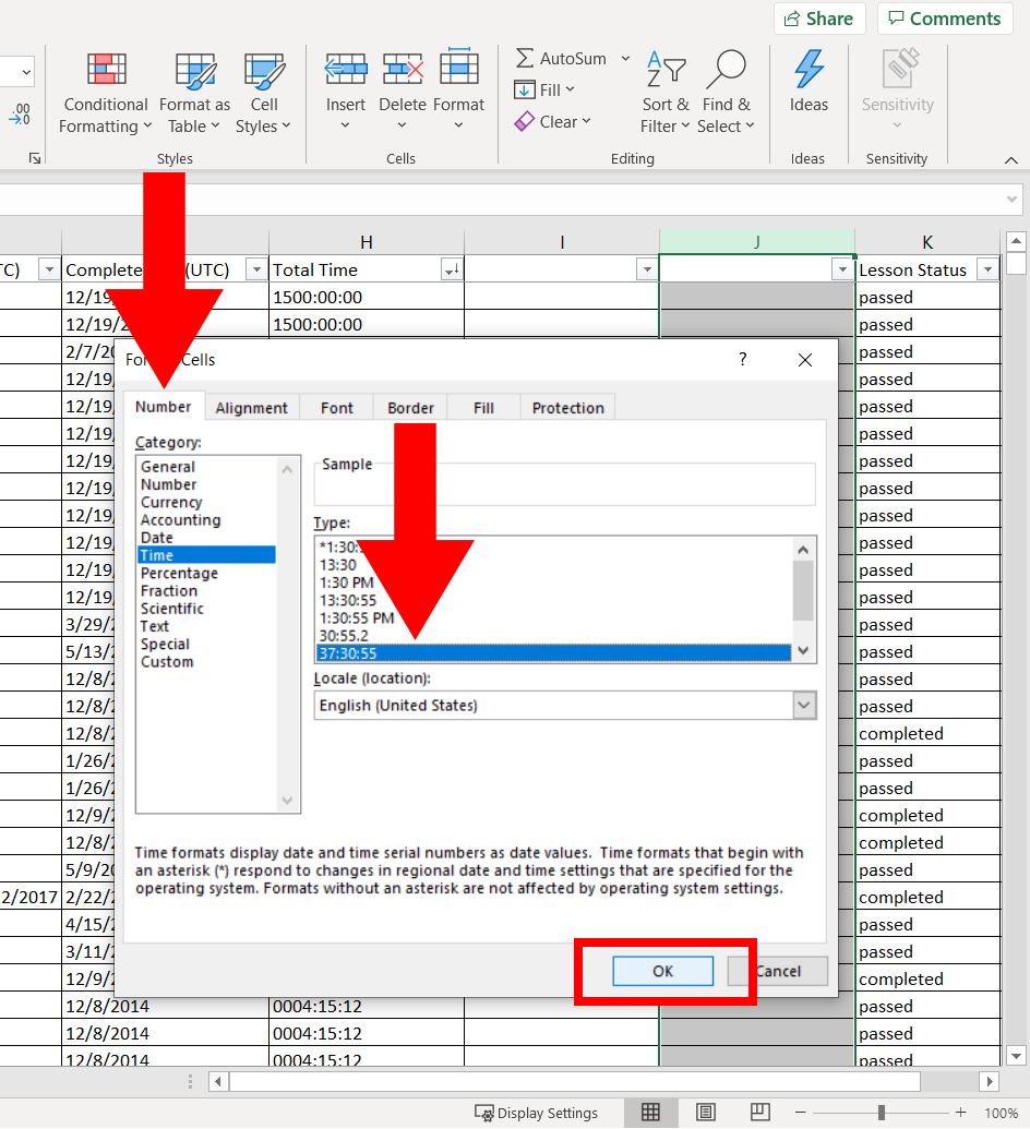
Format the second column to Time>37:30:55. Highlight the column, right click>Format Cell…>Number tab>Time>37:30:55>Ok
Use the following formula in the first column to the right of “Total Time” to remove the 2 leading zeros from all rows that are 0099:59:59 or less. Find the first record that is at most 0099:59:59, paste the formula =RIGHT(A1, LEN(A1)-2) into the cell and then adjusted the formula to align to your file’s columns and cells.
In this example the formula needed to be =RIGHT(H8, LEN(H8)-2)

Drag the formula down to the end of the report.
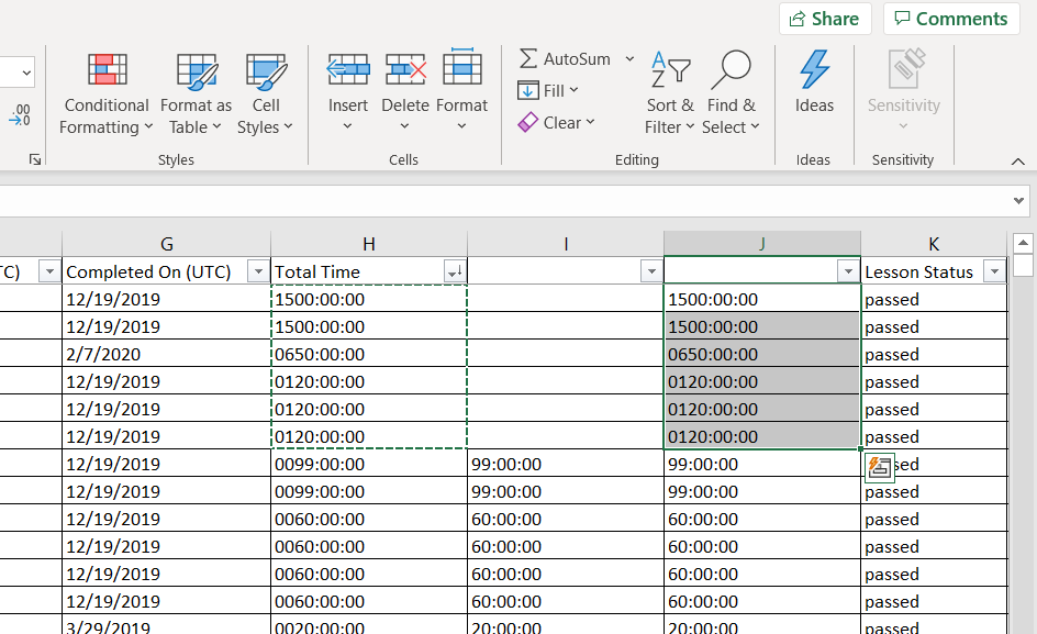
Select all the cells in the column (Shift+End+Down Arrow), then paste the Values into the next column to the right, line up to paste to the formula cell. In the example file that was J8.

If using the Excel export type, copy the longer times, paste Value into the column that now has the adjusted time values.
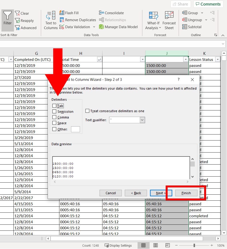
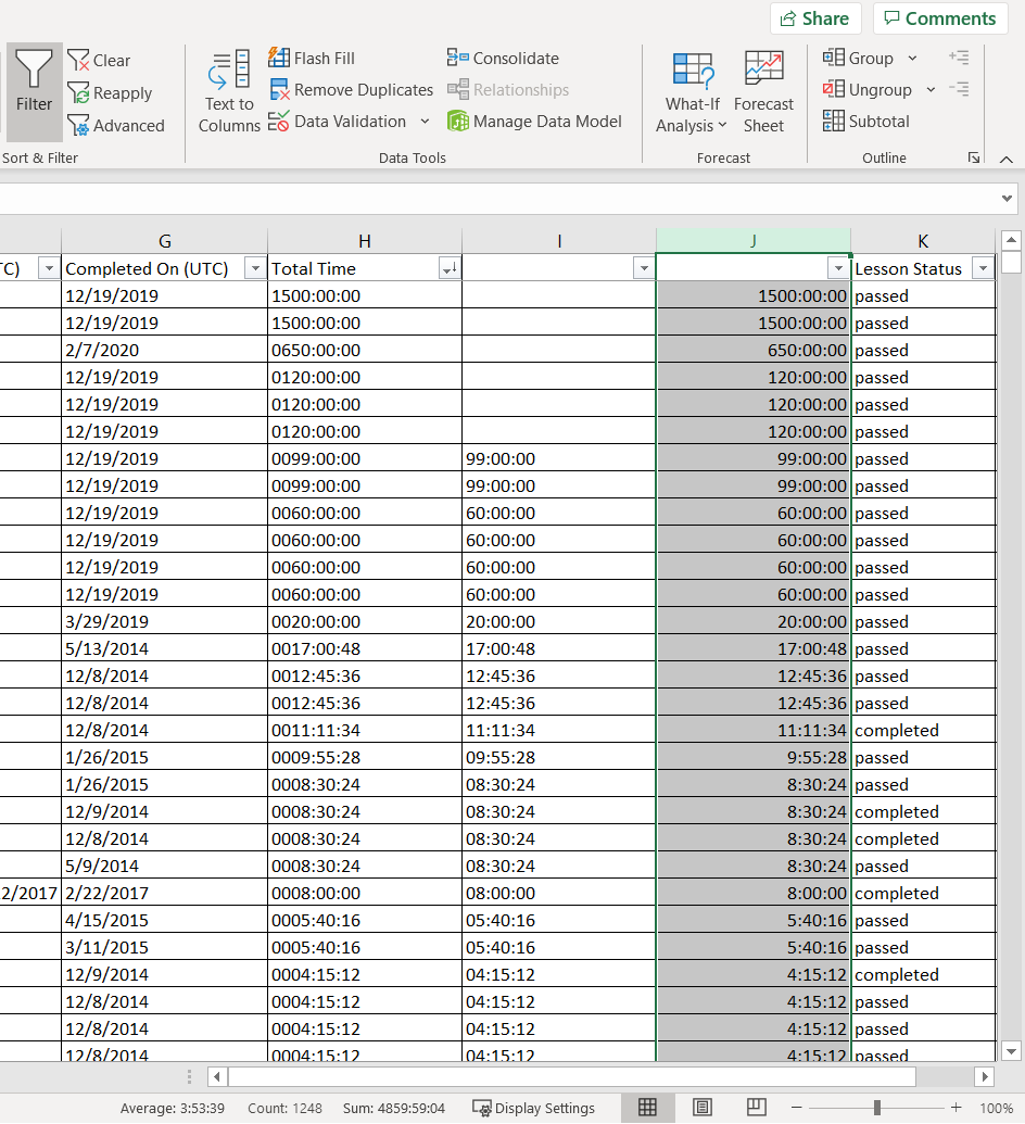
Last, highlight the whole column with the new values, go to the Data tab, then “Text to Column.” Select Delimited>Next>Remove all Delimiters>Finish. This should change the values into time that can be summed, averaged, etc.